Tutorial 2: Drawing Curves (Procedural Modelling)

Axes

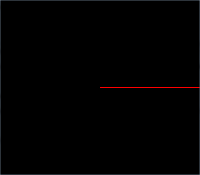
• Using the circle drawing code from the lecture extend to code to draw a set of 3 dimensional (3D) axes using GL_LINES, of length 1, making the x, y and z axis red, green and blue respectively. The z axis is pointing straight at the viewer, and so cant (easily) be seen. Have the centre of the axes at the world origin (0, 0, 0).
• Drawing axes is a fundamental educational technique and essential for visual debugging. As in normal good programming practice this code is written as a function so it can easily be reused. It could be put in a separate file.

Linear functions

A linear function has the general form y = mx + c where m is the gradient, and c is a constant and the y intercept. A portion of the line can be drawn as a line segment between two points on the line, from point P₁(x₁,y₁) to point P₂(x₂,y₂). Choose two x values x₁ and x₂ and work out the corresponding y values y₁ and y₂ using the equation of the line. For the tutorial we are still using the default OpenGL viewing system which provides coordinates which range over the interval [-1,1] in both x and y.

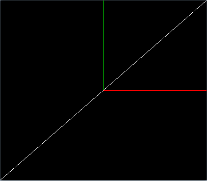
• Draw the function y = x
• Draw the function y = 2x + 1
• Draw the function y = -x/2

Quadratic functions

A quadratic function of the general form y=ax²+bx+c must be drawn as a series of connected straight line segments as OpenGL does not support directly drawing curved lines (or surfaces). Sometimes this is referred to as piecewise linear approximation (and in 3D curved surfaces are approximated by flat polygons). In mathematics the straight line segments joining points on the curve are sometimes referred to as chords. The drawing can be achieved using a for loop, where each iteration of the loop draws a single line segment. The more line segments used the better the approximation and the more curved the line looks, until we can’t tell the difference more segments make (and remembering the display is actually composed of pixels). Naturally better appearance from more segments comes at the cost of more work or computation.

• Write a for loop to iterate from 0 to the number of segments (inclusive).
• Calculate the step size for each segment as follows: left = -1.0, right = 1.0, range = right - left, stepSize = range / segments.
• Inside the body of the loop, calculate the current x value based on the current iteration: x = i × stepSize + left.
• Now inside the loop, using the x value you have calculated, draw a line segment for the function y = x. To make this easier, draw using GL_LINE_STRIP, that way you will only need one call to glVertex3f inside the loop.
• Now draw the other linear functions you implemented above. Confirm that they all look correct.
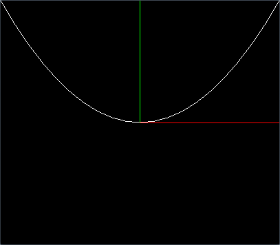
• Now draw the function y = x². You may find it easier to write a function float calculateFunction(float x) that you can call from inside the loop, to calculate the y value of any function you want with respect to x.
• Try changing the value of segments to make the curve smoother.
• Now draw the function y = 2x² - 1.
• Now draw the function y = -2x² + 2x + 1. Can you see the full curve? Should you be able to? If you are unsure of what these functions should look like type them into wolframalpha.

It may be useful to think of the above functions as parametric equations of the form:

x(t) = t, y(t) = t²

Where in this case t will be the current value you have calculated based on the number of segments.

Sine Waves

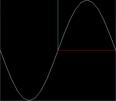
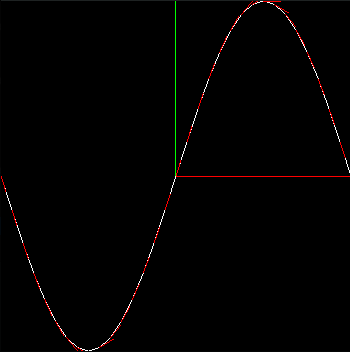
• Now create a function that draws a sine wave using the same technique. Use the function y = A * sin(k * x), where A is the amplitude and k = 2π / λ (λ is the wavelength). So in the image above to draw one wavelength in the interval -1 ≤ x ≤ 1, A = 1, λ = 2 and k = π. To get the value of π use M_PI available in math.h. Alternatively you can hard-code the value or initialise const float pi = 4.0 * atan(1.0) and use C++ i.e. g++ as non-constant initialisation is not allowed in C.
• Remember that the default OpenGL viewing system we are using has as x range of [-1,1], which means a wavelength of 2 in the image above. Try adjusting the wavelength and amplitude and see how it affects your sine wave. For example, for a wavelength λ = 1 instead of λ = 2, what is the value of k and what effect does it have?

Tangent Vectors

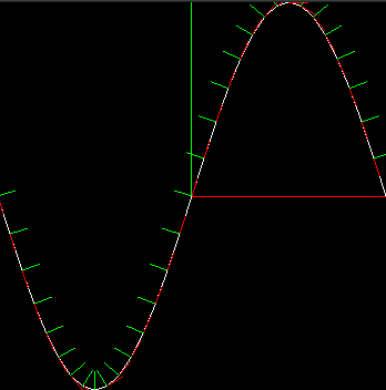
A tangent vector is a vector parallel to a curve (or surface) at a given point. It can be thought of pointing along the tangent line, the gradient m which can be calculated using the derivative dy/dx whereby T=<1,dy/dx>. The tangent vector can approximated by taking the average of two vectors: from the previous point to the current and the current to the next, or similarly using the average of the two gradients as an approximation to dy/dx.

• Write a function void drawVector(float x, float y, float a, float b, float s, bool normalize, float r, float g, float b) which draws as a line a vector <a, b> at (x, y) scaled by s, normalized depending of the value of normalize, in the color (r, g, b). First work out what the end point of the vector is - hint, use vector addition.
• To normalize a vector V means make its magnitude |V|=1, i.e. give it a length 1. To normalise a vector V=<a,b>, divide each component by the vector’s magnitude |V| = √(a²+b²) so V/|V| = <a/|V|,b/|V|>.
• Calculate the tangent T=<1, dy/dx> where y=sin(x). What is d(sin(x))/dx? Calculate and draw the tangent vector at (0,0), using drawVector with suitable parameters. Given the whole window is [-1,1] in x and y, the tangent vectors need to be drawn smaller, e.g. 0.1 - adjust the length of the vector using the parameter s.
• Now try drawing a tangent vector at every vertex. You will need to have another separate loop for this (otherwise the vectors become part of the line strip), even though it is basically the same as the loop for drawing the sine wave.

Normal Vectors

A normal vector is a vector perpendicular to a curve (or surface) at a given point. It can be calculated using the cross product of two tangent vectors (eg, one in the x direction and one in the z direction). For a simple 2d normal vector, after finding the tangent simply reverse the arguments and flip the sign of the new x value (eg tangent x, y becomes -y, x for the normal).

• Use drawVector to draw a normal vector at (0,0). Calculate it by hand and hard-code.
• Now calculate and draw the normal at each vertex.
• Try drawing the tangent and normal vectors for different curves, e.g. the quadratic. Confirm that they form a right angle at the point where they meet on the curve (this may look distorted depending on the aspect ratio).

Approximate Numerical Approach

• Try calculating the tangent and normals using the approximate numerical approach, that is, calculate the previous and next points on the curve and find the average. To draw this as a line you start the line at the current point (to start draw the tangent for the x value for testing) and add that point to your tangent for the end point.