Tutorial: 3D Sinewave with Lighting and Materials

Note: this web page uses MathML, mathematics markup for the web. We have installed mathjax which should render the MathML, But if the maths rendering looks broken, try Firefox, as it has strong MathML support. Chrome/Chromium support is being introduced

A Grid with Normals

A wireframe grid rendered in perspective, with normal vectors at each point

Start with your scene viewer code from last week.

Add a set of x, y, z axes if you don't already have one in the scene

Draw a single white line along the x axis broken into n (use n = 8) parts:

        
          xStep = 2.0 / n;
          glBegin(GL_LINE_STRIP);
          for (int i = 0; i <= n; i++) {
            /* What is this calculation doing? */
            x = -1.0 + i * xStep;
            glVertex3f(x, 0.0, 0.0);          
          }

Now draw a single row of the grid using a triangle strip - use a strip primitive rather than individual triangles. For each x value there will now be two z values (and use the [0,1] orthographic view volume). Output two vertices for each iteration of the loop. Set the polygon mode to wireframe, glPolygonMode(GL_FRONT_AND_BACK, GL_LINE);

Now draw an 8X8 grid on the xz plane - the normal way the axes are oriented in computer graphics, with z out of the screen and origin bottom left. Note that this means y is up, whereas most of mathematics usually has z up.

Again use quad or triangle strips, with one strip for each row. But now another outer loop needs to be added, similar to those in the lecture notes:

        
          xStep = 2.0 / n;                
          zStep = 2.0 / n; // xStep and zStep are the same, but could be different
          for (int j = 0; j < n; j++) {
            glBegin(GL_TRIANGLE_STRIP);
            z = -1.0 + j * zStep;
            for (int i = 0; i <= n; i++) {
              /* What are these calculations doing? */
              x = -1.0 + i * xStep;
              glVertex3f(...);
              // Replace this comment with calculation to work out next z value
              glVertex3f(...);
            }
            glEnd();                 
          }

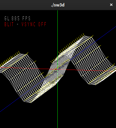
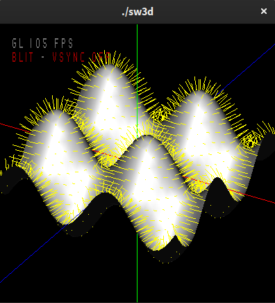
At each vertex on the grid, draw a yellow line pointing straight up on the y axis representing the normal. Use a function drawVector for this, as per previous tutorials.

Experiment with using a quad strip instead of a triangle strip. Only the glBegin should need changing. In the rendering pipeline polygons get turned in to triangles at some stage - GPUs are designed to render triangles rather than general polygons (and points and lines and some other non-polygon primitives)

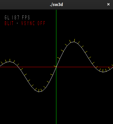
Extruded sine wave function

2D sine wave The same grid as above, with a sine wave applied along the x axis

Now, using the sine wave function y = A * sin(k * x) from tutorial 2, calculate the height of each point on the grid (its y value) so that it uses the sine function along the x axis. This should make it appear as a wave. Decrease the amplitude e.g. 0.25 so the wave is not so large. Adjust the normal vectors to start at the vertex points on the wave, if they no longer do.

If after changing the wave amplitude the normal vectors are not pointing in the correct direction, using the normal code from tutorial 2, try to render correct normals at each point on the grid. Visually confirm that they are pointing the right direction.

Add a key binding 'p' to toggle between filled and wireframe modes, add an 'n' option to toggle normal vector visualisation on/off.

Tangents

Sine wave
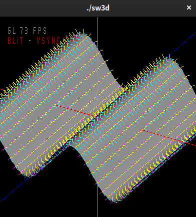
with tangent and binormal vectors

Now render the tangent vectors in the same way as the normal vectors, using the above technique. Now that the sine wave is a surface and not a curve, instead of just a tangent in the xy plane, there is also a tangent vector in the yz plane.

From the lecture notes on normals:

\begin{matrix} T_{xy} = < 1, \frac{\partial y}{\partial x}, 0 > \\ T_{yz} = < 0, \frac{\partial y}{\partial z}, 1 > \end{matrix}

The equation of the sine wave is, as above, y = A * sin(k * x). So $T_{xy} = < 1, \frac{\partial y}{\partial x}, 0 > = < 1, k A \cos (k x), 0 >$ That is really just the same as for 2D.

Also, as y only depends on x, z is not in the equation for y, then $\frac{\partial y}{\partial z} = 0$ and $T_{yz} = < 0, 0, 1 >$

Back to the wave rendering. Add 't' and 'b' keys to toggle tangent visualisation in the xy and yz planes.

Lighting

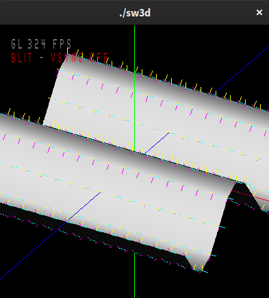
The same grid as above, filled, with correct lighting

Once the normal vectors are correct, call glNormal3f(...) before each glVertex call. Just like glColor, glNormal sets the normal to be used for successive glVertex calls. Make sure to turn wireframe off, so the grid is drawn with filled polygons and the effects of the lighting can be seen. Enable lighting with the following functions:

	
	  glEnable(GL_LIGHTING);
          glEnable(GL_LIGHT0);

This will also enable lighting for all objects including lines, so make sure to disable it before drawing the axes, and re-enable it afterward.
What happens when the normals are scaled so they are not unit length? Add glEnable(GL_NORMALIZE); so OpenGL will normalize normals before the lighting calculations are performed. If normals are already normalized, is GL_NORMALIZE required? When would it be required?
What direction is the light coming from? Set the position of the light using glLightfv(...) for GL_LIGHT0 with a GL_POSITION of (1,1,1,0).

Extra:

You can use glLightfv to set the lights diffuse, ambient and specular colors, as well as its shininess.

Materials

Now set the material properties for the grid. For debugging purposes, set the properties for GL_FRONT_AND_BACK. Using glMaterialfv, first set the ambient, diffuse colours using glMaterialfv(GL_FRONT_AND_BACK, GL_AMBIENT_AND_DIFFUSE, cyan) where cyan is a color3f (which is just another name for a vec3f using a typedef) storing the color value cyan (0,1,1). Now try adding a white specular color to give white highlights. Change these values and see how it affects the grid. * Using glMaterialf, set the shininess to 50. Change this value, what happens?

Extra:

What happens when you also change these values for glLightfv? How do they combine to produce the final color for the grid?

Animated 3D sine wave

Now try animating the 3D sine wave using the function y = A * sin(k * x + w * t), as in tutorial 2 and the first assignment. Animated 3D waves are required in the second assignment.

Code Refactoring

Modify your code:

use a typedef to define a sinewave type using a struct which stores the parameters of a sine wave: A, k and w
use a global variable sw to store a sinewave with values A = ¼, k = 2 * π, w = ¼π.
define and use a function void calcSineWave(sinewave sw, float x, float t, float *y, bool dvs, float *dydx) The argument dvs indicates whether the derivative is to be calculated, which is used in the normal and tangent calculation.
A flag controlling the derivative calculation is a good example of considerations about performance. The derivative is a reasonably expensive calculation involving trig functions. It is only needed if normals are being visualised or if lighting is enabled - which requires normals, or tangents are being visualised. Managing these kinds of optimisations with switches and flags is an important technique in rendering performance improvement. But it leads to quite tricky code with different rendering paths very quickly!

More Complex Wave Forms

Muliple sine waves can be added together to create more complex wave forms, e.g. to better resemble water waves.

Implement a function calcSineWaveSum which takes an array of sine waves and adds them up by calling calcSineWave. Just add the y values up for all sine waves. Try two sine waves:

A = ¼, k = 2 * π, w = ¼π and
A = ¼, k = π, w = ½π.

And Yet More Complex Wave Forms

So far the waves have had the form y = A * sin(k * x + w * t) - and the y values do not depend i.e. vary with z, as z is not in the equation. Try y = A * sin(k * z + w * t). Now the wave depends on z but not x. Be careful about calculations of x, y and z to make sure the wave is continuous and does not have gaps.

A wave equation which varies with x and z, as well as t is y = A * sin(kx * x + kz * z + w * t)

Experiment! Try equal values for kx and kz. Note that for this curve the derivative in the yz plane is not zero. Getting the normals, and thus the lighting, right is tougher!